Machine Learning Concepts

This post covers some of the basic Machine Learning concepts mostly relevant for the AWS AI and Machine Learning certification exams.

Machine Learning Lifecycle

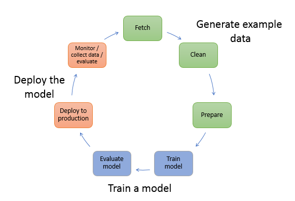
Data Processing and Exploratory Analysis

• To train a model, you need data.
• Type of data that depends on the business problem that you want the model to solve (the inferences that you want the model to generate).
• Process data includes data collection, data cleaning, data split, data exploring, preprocessing, transformation, formatting etc.

Feature Selection and Engineering

• helps improve model accuracy and speed up training
• remove irrelevant data inputs using domain knowledge for e.g. name
• remove features which has same values, very low correlation, very little variance or lot of missing values
• handle missing data using mean values or imputation
• combine features which are related for e.g. height and age to height/age
• convert or transform features to useful representation for e.g. date to day or hour
• standardize data ranges across features

Missing Data

• do nothing
• remove the feature with lot of missing data points
• remove samples with missing data, if the feature needs to be used
• Impute using mean/median value
  • no impact and the dataset is not skewed
  • works with numerical values only. Do not use for categorical features.
  • doesn’t factor correlations between features
• Impute using (Most Frequent) or (Zero/Constant) Values
  • works with categorical features
  • doesn’t factor correlations between features
  • can introduce bias
• Impute using k-NN, Multivariate Imputation by Chained Equation (MICE), Deep Learning
  • more accurate than the mean, median or most frequent
  • Computationally expensive

Unbalanced Data

• Source more real data
• Oversampling instances of the minority class or undersampling instances of the majority class
• Create or synthesize data using techniques like SMOTE (Synthetic Minority Oversampling TEchnique)

Label Encoding and One-hot Encoding

• Models cannot multiply strings by the learned weights, encoding helps convert strings to numeric values.
• Label encoding
  • Use Label encoding to provide lookup or map string data values to a numerical values
  • However, the values are random and would impact the model
• One-hot encoding
  • Use One-hot encoding for Categorical features that have a discrete set of possible values.
  • One-hot encoding provide binary representation by converting data values into features without impacting the relationships
  • a binary vector is created for each categorical feature in the model that represents values as follows:
    • For values that apply to the example, set corresponding vector elements to 1.
    • Set all other elements to 0.
  • Multi-hot encoding is when multiple values are 1

Cleaning Data

• Scaling or Normalization means converting floating-point feature values from their natural range (for example, 100 to 900) into a standard range (for example, 0 to 1 or -1 to +1)

Train a model

• Model training includes both training and evaluating the model,
• To train a model, algorithm is needed.
• Data can be split into training data, validation data and test data
  • Algorithm sees and is directly influenced by the training data
  • Algorithm uses but is indirectly influenced by the validation data
  • Algorithm does not see the testing data during training
• Training can be performed using normal parameters or features and hyperparameters

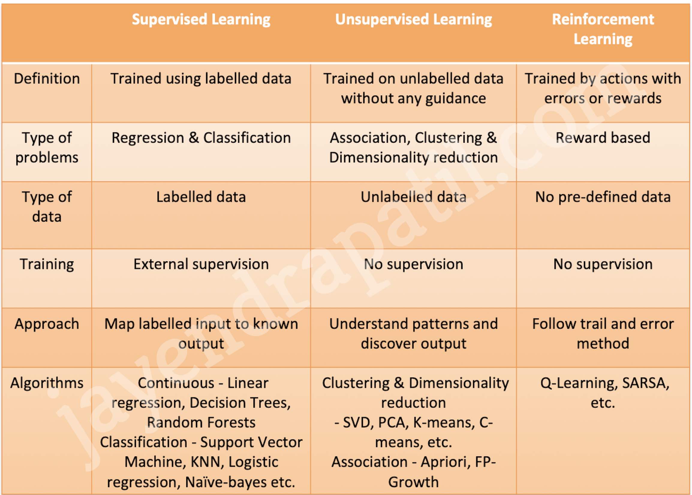
Supervised, Unsupervised, Semi-Supervised, and Reinforcement Learning

Supervised Learning

• Uses labeled data — both input features and correct output (target) are provided
• Model learns mapping between inputs and outputs
• Types: Classification (categorical output) and Regression (continuous output)
• Examples: spam detection, image classification, price prediction

Unsupervised Learning

• Uses unlabeled data — no target variable provided
• Model discovers hidden patterns or structures in data
• Types: Clustering, Dimensionality Reduction, Anomaly Detection, Association
• Examples: customer segmentation, PCA, anomaly detection

Semi-Supervised Learning

• Combines a small amount of labeled data with a large amount of unlabeled data
• Useful when labeling data is expensive or time-consuming
• The model learns from labeled data and generalizes using unlabeled data patterns
• Examples: medical image classification (few expert-labeled images + many unlabeled)

Self-Supervised Learning

• A form of unsupervised learning where the model generates its own labels from the input data
• The foundation of modern Large Language Models (LLMs) and Foundation Models
• Techniques include masked language modeling (predict missing words) and next-token prediction
• Enables pre-training on massive unlabeled datasets before fine-tuning on specific tasks
• Examples: BERT (masked word prediction), GPT (next-token prediction)

Reinforcement Learning

• Agent learns by interacting with an environment and receiving rewards or penalties
• Goal is to maximize cumulative reward through trial and error
• Key concepts: Agent, Environment, State, Action, Reward, Policy
• Used in robotics, game playing, autonomous vehicles, recommendation systems
• Reinforcement Learning from Human Feedback (RLHF) — used to fine-tune LLMs based on human preference rankings (key technique behind ChatGPT and similar models)

Splitting and Randomization

• Always randomize the data before splitting

Hyperparameters

• influence how the training occurs
• Common hyperparameters are learning rate, epoch, batch size
• Learning rate
  • size of the step taken during gradient descent optimization
  • Large learning rates can overshoot the correct solution
  • Small learning rates increase training time
• Batch size
  • number of samples used to train at any one time
  • can be all (batch), one (stochastic), or some (mini-batch)
  • calculable from infrastructure
  • Small batch sizes tend to not get stuck in local minima
  • Large batch sizes can converge on the wrong solution at random.
• Epochs
  • number of times the algorithm processes the entire training data
  • each epoch or run can see the model get closer to the desired state
• depends on algorithm used

Evaluating the model

After training the model, evaluate it to determine whether the accuracy of the inferences is acceptable.

ML Model Insights

• For binary classification models use accuracy metric called Area Under the (Receiver Operating Characteristic) Curve (AUC). AUC measures the ability of the model to predict a higher score for positive examples as compared to negative examples.
• For regression tasks, use the industry standard root mean square error (RMSE) metric. It is a distance measure between the predicted numeric target and the actual numeric answer (ground truth). The smaller the value of the RMSE, the better is the predictive accuracy of the model.

Cross-Validation

• is a technique for evaluating ML models by training several ML models on subsets of the available input data and evaluating them on the complementary subset of the data.
• Use cross-validation to detect overfitting, ie, failing to generalize a pattern.
• there is no separate validation data, involves splitting the training data into chunks of validation data and use it for validation

Optimization

• Gradient Descent is used to optimize many different types of machine learning algorithms
• Step size sets Learning rate
  • If the learning rate is too large, the minimum slope might be missed and the graph would oscillate
  • If the learning rate is too small, it requires too many steps which would take the process longer and is less efficient

Underfitting

• Model is underfitting the training data when the model performs poorly on the training data because the model is unable to capture the relationship between the input examples (often called X) and the target values (often called Y).
• To increase model flexibility
  • Add new domain-specific features and more feature Cartesian products, and change the types of feature processing used (e.g., increasing n-grams size)
  • Regularization – Decrease the amount of regularization used
  • Increase the amount of training data examples.
  • Increase the number of passes on the existing training data.

Overfitting

• Model is overfitting the training data when the model performs well on the training data but does not perform well on the evaluation data because the model is memorizing the data it has seen and is unable to generalize to unseen examples.
• To increase model flexibility
  • Feature selection: consider using fewer feature combinations, decrease n-grams size, and decrease the number of numeric attribute bins.
  • Simplify the model, by reducing the number of layers.
  • Regularization – technique to reduce the complexity of the model. Increase the amount of regularization used.
  • Early Stopping – a form of regularization while training a model with an iterative method, such as gradient descent.
  • Data Augmentation – process of artificially generating new data from existing data, primarily to train new ML models.
  • Dropout is a regularization technique that prevents overfitting.

Deep Learning and Neural Networks

• Deep Learning is a subset of machine learning that uses neural networks with multiple layers (deep neural networks) to learn complex patterns
• Excels at tasks involving unstructured data (images, text, audio)
• Requires large amounts of data and significant compute resources

Neural Network Fundamentals

• Composed of layers: Input Layer, Hidden Layers, and Output Layer
• Each neuron applies weights, bias, and an activation function to its inputs
• Common activation functions: ReLU, Sigmoid, Tanh, Softmax
• Backpropagation — algorithm used to calculate gradients and update weights during training
• A network with 2+ hidden layers is considered a “deep” neural network

Types of Neural Networks

Convolutional Neural Networks (CNNs)

• Specialized for processing grid-like data (images, spatial data)
• Uses convolutional layers with filters/kernels to detect features (edges, shapes, objects)
• Key layers: Convolutional, Pooling (Max/Average), Fully Connected
• Use cases: image classification, object detection, computer vision

Recurrent Neural Networks (RNNs)

• Designed for sequential data (time series, text, speech)
• Maintains internal state (memory) that captures information from previous time steps
• LSTM (Long Short-Term Memory) — addresses vanishing gradient problem with gates (forget, input, output)
• GRU (Gated Recurrent Unit) — simplified version of LSTM with fewer parameters
• Largely superseded by Transformers for NLP tasks due to inability to parallelize

Transformers

• Architecture introduced in “Attention Is All You Need” (2017) — foundation of modern LLMs
• Processes entire input sequences in parallel using self-attention mechanism
• Key innovation: Attention mechanism allows each token to attend to every other token regardless of distance
• Components: Multi-Head Attention, Positional Encoding, Feed-Forward Layers, Layer Normalization
• Encoder — processes input and creates representations (BERT-style models)
• Decoder — generates output tokens auto-regressively (GPT-style models)
• Encoder-Decoder — used for sequence-to-sequence tasks (T5, translation)
• Use cases: NLP, text generation, translation, code generation, image generation

Generative Adversarial Networks (GANs)

• Two networks compete: Generator (creates synthetic data) vs Discriminator (detects fake data)
• Training improves both networks iteratively
• Use cases: image generation, style transfer, data augmentation

Generative AI and Foundation Models

• Generative AI is a subset of deep learning that creates new content (text, images, code, audio, video) based on patterns learned from training data
• Foundation Models (FMs) are large pre-trained models trained on broad datasets that can be adapted for many downstream tasks
• Examples: GPT-4, Claude, Amazon Titan, Amazon Nova, Llama, Gemini

Large Language Models (LLMs)

• Foundation models trained on massive text corpora using self-supervised learning
• Based on the Transformer architecture
• Capabilities: text generation, summarization, translation, code generation, reasoning
• Key characteristics:
  • Parameters — learned weights (billions to trillions); more parameters generally = more capability
  • Context window — maximum number of tokens the model can process at once
  • Tokens — basic units of text (words or sub-words) the model processes
  • Temperature — controls randomness of output (0 = deterministic, higher = more creative)

Customizing Foundation Models

Prompt Engineering

• Crafting input prompts to guide model output without changing model weights
• Zero-shot — no examples provided in prompt
• Few-shot — providing examples in the prompt to guide the response
• Chain-of-thought — guiding model to show reasoning steps
• No training required; fastest and cheapest customization method

Retrieval-Augmented Generation (RAG)

• Combines retrieval of external knowledge with generation of responses
• Retrieves relevant documents from a knowledge base and includes them in the prompt context
• Reduces hallucinations by grounding responses in factual data
• No model retraining required; knowledge base can be updated independently
• Components: Document store, Embedding model, Vector database, Retriever, Generator
• AWS service: Amazon Bedrock Knowledge Bases

Fine-Tuning

• Further training a pre-trained model on a task-specific labeled dataset
• Updates model weights to specialize for specific domain or task
• Requires labeled training data and compute resources
• Types:
  • Full fine-tuning — updates all model parameters (expensive)
  • Parameter-Efficient Fine-Tuning (PEFT) — updates only a small subset of parameters
  • LoRA (Low-Rank Adaptation) — adds small trainable matrices to frozen model layers
• AWS service: Amazon Bedrock and Amazon SageMaker AI

Continued Pre-Training

• Training a foundation model on additional domain-specific unlabeled data
• Teaches the model new domain knowledge (medical, legal, financial terminology)
• More expensive than fine-tuning but creates deeper domain understanding

Transfer Learning

• Technique of using a model trained on one task as the starting point for a related task
• Reduces training time and data requirements significantly
• Foundation models are the ultimate form of transfer learning — pre-trained on broad data, then adapted
• Approaches: Feature extraction (freeze base layers) or Fine-tuning (update some/all layers)

Agentic AI

• AI systems that can autonomously plan, reason, and take actions to accomplish goals
• Uses tools, APIs, and knowledge bases to complete multi-step tasks
• Key components: Planning, Memory, Tool use, Reasoning
• AWS service: Amazon Bedrock Agents, Amazon Bedrock AgentCore

Classification Model Evaluation

Confusion Matrix

• Confusion matrix represents the percentage of times each label was predicted in the training set during evaluation
• An NxN table that summarizes how successful a classification model’s predictions were; that is, the correlation between the label and the model’s classification.
• One axis of a confusion matrix is the label that the model predicted, and the other axis is the actual label.
• N represents the number of classes. In a binary classification problem, N=2
  • For example, here is a sample confusion matrix for a binary classification problem:

	Tumor (predicted)	Non-Tumor (predicted)
Tumor (actual)	18 (True Positives)	1 (False Negatives)
Non-Tumor (actual)	6 (False Positives)	452 (True Negatives)

• • Confusion matrix shows that of the 19 samples that actually had tumors, the model correctly classified 18 as having tumors (18 true positives), and incorrectly classified 1 as not having a tumor (1 false negative).
  • Similarly, of 458 samples that actually did not have tumors, 452 were correctly classified (452 true negatives) and 6 were incorrectly classified (6 false positives).
• Confusion matrix for a multi-class classification problem can help you determine mistake patterns. For example, a confusion matrix could reveal that a model trained to recognize handwritten digits tends to mistakenly predict 9 instead of 4, or 1 instead of 7.

Accuracy, Precision, Recall (Sensitivity) and Specificity

Accuracy

• A metric for classification models, that identifies fraction of predictions that a classification model got right.
• In Binary classification, calculated as (True Positives+True Negatives)/Total Number Of Examples
• In Multi-class classification, calculated as Correct Predictions/Total Number Of Examples

Precision

• A metric for classification models. that identifies the frequency with which a model was correct when predicting the positive class.
• Calculated as True Positives/(True Positives + False Positives)

Recall – Sensitivity – True Positive Rate (TPR)

• A metric for classification models that answers the following question: Out of all the possible positive labels, how many did the model correctly identify i.e. Number of correct positives out of actual positive results
• Calculated as True Positives/(True Positives + False Negatives)
• Important when – False Positives are acceptable as long as ALL positives are found for e.g. it is fine to predict Non-Tumor as Tumor as long as All the Tumors are correctly predicted

Specificity – True Negative Rate (TNR)

• Number of correct negatives out of actual negative results
• Calculated as True Negatives/(True Negatives + False Positives)
• Important when – False Positives are unacceptable; it’s better to have false negatives for e.g. it is not fine to predict Non-Tumor as Tumor;

ROC and AUC

ROC (Receiver Operating Characteristic) Curve

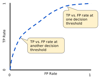
• An ROC curve (receiver operating characteristic curve) is curve of true positive rate vs. false positive rate at different classification thresholds.
• An ROC curve is a graph showing the performance of a classification model at all classification thresholds.
• An ROC curve plots True Positive Rate (TPR) vs. False Positive Rate (FPR) at different classification thresholds. Lowering the classification threshold classifies more items as positive, thus increasing both False Positives and True Positives.

  

AUC (Area under the ROC curve)

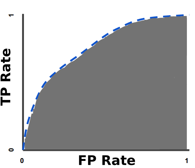
• AUC stands for “Area under the ROC Curve.”
• AUC measures the entire two-dimensional area underneath the entire ROC curve (think integral calculus) from (0,0) to (1,1).
• AUC provides an aggregate measure of performance across all possible classification thresholds.
• One way of interpreting AUC is as the probability that the model ranks a random positive example more highly than a random negative example.

F1 Score

• F₁ score (also F-score or F-measure) is a measure of a test’s accuracy.
• It considers both the precision p and the recall r of the test to compute the score: p is the number of correct positive results divided by the number of all positive results returned by the classifier, and r is the number of correct positive results divided by the number of all relevant samples (all samples that should have been identified as positive).
• Calculated as: F1 = 2 × (Precision × Recall) / (Precision + Recall)
• Ranges from 0 to 1, with 1 being perfect precision and recall
• Useful when you need a balance between precision and recall, especially with imbalanced datasets

Generative AI Evaluation Metrics

• Traditional ML metrics (accuracy, F1) are insufficient for evaluating generative AI outputs
• Generative AI requires metrics that measure quality, safety, relevance, and factual accuracy

Text Generation Metrics

BLEU (Bilingual Evaluation Understudy)

• Measures n-gram overlap between generated text and reference text
• Ranges from 0 to 1 (higher is better)
• Originally designed for machine translation evaluation
• Limitation: only measures lexical similarity, not semantic meaning

ROUGE (Recall-Oriented Understudy for Gisting Evaluation)

• Measures overlap between generated summary and reference summary
• ROUGE-N — n-gram overlap (ROUGE-1 = unigrams, ROUGE-2 = bigrams)
• ROUGE-L — longest common subsequence
• Commonly used for summarization tasks

Perplexity

• Measures how well a model predicts a sequence of words
• Lower perplexity = better model (model is less “surprised” by the text)
• Useful for comparing language models but doesn’t directly measure output quality

BERTScore

• Uses contextual embeddings to measure semantic similarity between generated and reference text
• Better than BLEU/ROUGE at capturing meaning rather than just word overlap

Generative AI Safety Metrics

Hallucination Rate

• Measures how often a model generates factually incorrect or fabricated information
• Critical metric for production deployments
• Mitigated by RAG, grounding, and guardrails

Groundedness

• Measures whether model responses are supported by provided context/source documents
• Key metric for RAG systems

Toxicity and Content Safety

• Measures presence of harmful, biased, or inappropriate content in outputs
• AWS service: Amazon Bedrock Guardrails for content filtering

Human Evaluation and LLM-as-a-Judge

• Human evaluation remains the gold standard for assessing quality, helpfulness, and safety
• LLM-as-a-Judge — using a capable LLM to evaluate outputs of another model (scalable alternative to human evaluation)
• AWS service: Amazon Bedrock Evaluations for automated model evaluation

Responsible AI and ML Fairness

• Ensuring AI systems are fair, transparent, accountable, and safe
• Regulatory frameworks: EU AI Act, ISO 42001, NIST AI RMF

Bias in Machine Learning

• Data Bias — bias present in training data (sampling bias, historical bias, measurement bias)
• Algorithmic Bias — bias introduced by the model or training process
• Selection Bias — non-representative training data
• Detection: AWS Amazon SageMaker Clarify provides pre-training and post-training bias detection metrics

Explainability and Interpretability

• Explainability — ability to understand why a model made a specific prediction
• Techniques: SHAP (SHapley Additive exPlanations), feature importance, attention visualization
• AWS service: Amazon SageMaker Clarify for model explainability
• Critical for regulated industries (healthcare, finance) where decisions must be justified

Model Governance

• Tracking model lineage, versioning, and approval workflows
• Model cards documenting intended use, limitations, and evaluation results
• AWS service: Amazon SageMaker Model Registry and SageMaker Data & AI Governance

Deploy the model

• Re-engineer a model before integrating it with the application and deploy it.
• Can be deployed as a Batch or as a Service (real-time endpoint)
• Model Monitoring — continuously track model performance in production to detect drift
  • Data Drift — input data distribution changes over time compared to training data
  • Model Drift (Concept Drift) — relationship between input and output changes over time
  • Requires retraining or updating the model when drift is detected
• A/B Testing — deploying multiple model variants to compare performance with real traffic
• Shadow Deployment — running new model alongside production model without serving its predictions to users

AWS Machine Learning Services Summary

• Amazon SageMaker AI — fully managed service to build, train, and deploy ML models at scale
• Amazon Bedrock — managed service to build generative AI applications using foundation models (Amazon Titan, Amazon Nova, Claude, Llama, etc.)
• Amazon Bedrock Knowledge Bases — managed RAG service
• Amazon Bedrock Agents — build autonomous AI agents
• Amazon Bedrock Guardrails — content filtering and safety controls
• Amazon Q Developer — AI-powered coding assistant
• Amazon SageMaker Clarify — bias detection and model explainability
• Amazon Comprehend — NLP service for text analysis
• Amazon Rekognition — computer vision service
• Amazon Transcribe — speech-to-text
• Amazon Polly — text-to-speech
• Amazon Translate — language translation

References

• AWS Machine Learning
• Amazon Bedrock
• Amazon SageMaker AI
• AWS – What is RAG?
• SageMaker Clarify – Bias Metrics
• AWS Certified AI Practitioner
• AWS Certified ML Engineer Associate